BESS Merchant Energy Arbitrage sounds simple on paper: charge when prices are low, discharge when prices are high, and pocket the spread. But if you’ve ever tried to translate that story into a lender-clean Excel model, you know the truth: Energy Arbitrage is rarely “buy low, sell high” in the real world. The economics are driven by a tight set of constraints—cycles, losses, deliverability, and price shapes—and if you don’t model those mechanics explicitly, your BESS Merchant Energy Arbitrage profits will almost always look better than what the asset can actually earn.

The problem isn’t that arbitrage doesn’t work. The problem is that most models skip the steps that turn a price spread into bankable cash flows. A realistic arbitrage engine has to answer four questions with precision:

1. How many cycles can the battery actually run?
   Equivalent Full Cycles (EFCs) are the control knob for throughput. A battery might be physically capable of cycling daily, but in many real structures—especially when the project also sells contracted capacity—dispatch flexibility is limited. Your arbitrage upside is then “headroom monetization,” not unlimited daily spread capture.

2. What price curve are you arbitraging—pure merchant or constrained?
   In real deals, you often cannot charge at the daily minimum and discharge at the peak. The price curves you’re allowed to monetize may be constrained by contractual obligations, grid rules, or operational priorities. If you ignore that, you are implicitly assuming a “perfect trader” battery—something lenders won’t finance.

3. How much energy do you buy vs. how much do you sell?
   Losses are not a footnote. Round-trip efficiency, one-way conversion losses, and transformer/MV losses determine the gap between energy required to charge and energy you can deliver back to the grid. A correct model forces you to compute both paths explicitly—and it keeps your accounting discipline clean across AC/DC boundaries.

4. Do availability and curtailment reduce merchant opportunity?
   If the battery is unavailable, you can’t arbitrage. If it’s curtailed, you might not be able to inject energy when spreads are attractive. Whether you embed those effects in the EFC assumption or model them as explicit adjustment switches, the key is consistency—no double-counting, no missing haircuts.

That’s exactly what we’ll build in this article: a practical BESS Merchant Energy Arbitrage revenue engine in Excel that starts with charge/discharge price forecasts, applies cycles and operational constraints, converts energy correctly through the efficiency stack, and outputs clean profit metrics—per cycle and per year—that you can actually use in project finance modeling.

The Excel Framework We’ll Build (Watch Deal Lab Part 6 First)

Before we go into the mechanics, it helps to be crystal clear on what “good” looks like in BESS Merchant Energy Arbitrage modeling. The goal isn’t to create a complicated spreadsheet—it’s to build a transparent, auditable engine that turns a spread story into numbers you can defend in an investment memo or a lender model review.

At a high level, the framework has four building blocks:

1. Merchant price inputs (charge & discharge)
   You need two time series: the average price you pay to charge and the average price you earn when discharging. In the Deal Lab model, these come from the Inputs Time Dependent sheet as annual forecasts (the kind of forecasts you’d typically receive from an independent market consultant). This is important: we’re not pretending we can simulate hourly dispatch inside a yearly project finance model. Instead, we create a clean container for forecast assumptions and build a disciplined translation to annual cash flows.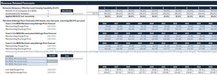

2. Throughput control via cycles (EFCs)
   Cycles per year are the throttle. If you assume too many cycles, your BESS Merchant Energy Arbitrage profit will look amazing—but it will be economically and operationally unrealistic. If you assume too few, you’ll understate upside. In our RA + Arbitrage case (Case 5), the cycles are intentionally constrained (120 EFC/year) because the battery is primarily committed to a capacity product, leaving limited headroom for spread capture.

3. Energy per cycle (charge vs discharge) with losses applied correctly
   This is where most models quietly break. You don’t “buy 1 MWh and sell 1 MWh.” You buy more than you sell, because losses sit in the conversion chain. In the model we explicitly compute:

• Energy required for a full charge (AC energy drawn from the grid, after switches for availability/curtailment if applicable)

• Usable energy delivered back (AC energy injected to the grid, after efficiency and loss adjustments)

That AC/DC boundary discipline matters because revenues settle at the point of interconnection on an AC basis, while physics and degradation live on the DC side. If your math blurs that line, your BESS Merchant Energy Arbitrage cash flows won’t be lender-clean.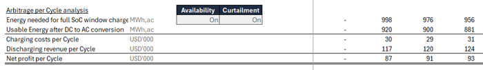

4. Cash flow outputs (per cycle and per year)
   Once we have prices and energy, the economics become simple and intuitive:

• Charging cost per cycle = charge price × charge energy

• Discharge revenue per cycle = discharge price × discharge energy

• Net profit per cycle = revenue − cost
  Then scale it: multiply by cycles/year to get annual costs, annual revenues, and annual gross profit.

To make this as practical as possible, we recommend watching the Deal Lab lesson first—then coming back to this article as your “mental model + written reference” while implementing it in Excel.

🎥 Deal Lab Part 6 — BESS Merchant Energy Arbitrage Model in Excel

In that video, you’ll see the full BESS Merchant Energy Arbitrage block built step-by-step: pulling charge/discharge price forecasts with XLOOKUP, converting real prices to nominal using an index selection, computing charge and discharge energy per cycle with the correct operational adjustments, and translating it all into annual profit that actually drives the dashboard revenue mix. Once you’ve watched it, the next section of this article will walk you through the key assumptions behind the RA-constrained arbitrage setup—so your BESS Merchant Energy Arbitrage doesn’t accidentally assume a “perfect merchant” battery that the contract structure simply doesn’t allow.

Why Arbitrage Needs a “Base Layer”: Resource Adequacy (RA), ELCC & NQC

If you want your merchant upside to feel realistic in a project finance model, you need to start from the constraint, not from the spread. In Project Pulse Case 5, the battery isn’t a free-floating merchant trader—it’s a 4-hour resource adequacy asset first, with merchant arbitrage layered on top. That’s exactly why the Deal Lab uses a deliberately modest arbitrage throughput assumption (120 equivalent full cycles per year): the project has RA obligations, and arbitrage is only monetized with the headroom that remains.

This context matters for BESS Merchant Energy Arbitrage because it changes both the economics and the credibility of the assumptions. In many markets, the RA payment is tied to the part of the battery that is accredited as reliable capacity. That accredited slice is not equal to 100% of nameplate forever. Instead, it’s governed by ELCC (Effective Load Carrying Capability), which is typically modeled as a time-dependent percentage that trends down as the grid becomes more saturated with storage.

The key idea in one sentence

A tolling contract pays for the battery’s contracted capacity directly, but an RA contract pays for net qualifying capacity (NQC)—the portion of nameplate that counts as reliable, which is nameplate × ELCC (and then adjusted for availability and other contract specifics).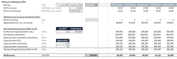

In the model, this “base layer” is implemented cleanly and transparently:

• You reuse most of the tolling agreement structure (flag, term, price, indexation, capacity basis).

• Then you add what’s RA-specific:

  • a RA year counter (so you can map year 1–20 to an ELCC path),

  • an XLOOKUP-based ELCC time series (often provided by a market consultant),

  • and the NQC calculation that determines what actually earns the RA payment.

Why do we care in a merchant-focused article? Because once you understand the RA base layer, you understand why the arbitrage overlay is constrained, why the “perfect spread capture” assumption is wrong, and why a realistic BESS Merchant Energy Arbitrage model must reflect product priorities (RA first, merchant second). The RA revenue stabilizes the project and makes the structure more financeable, while arbitrage becomes the upside option that can improve equity returns without being fully underwritten for debt sizing.

🎥 Deal Lab Part 5 — BESS Resource Adequacy (RA) Revenue Model in Excel

In Part 5, you’ll see the RA block built on the operations sheet: starting from contract terms and a fixed $/kW-month capacity payment, then layering in ELCC to convert nameplate AC capacity into NQC, and finally translating that into annual contracted cash flows. Once that base layer is in place, the merchant overlay in Part 6 becomes far more defensible—because your BESS Merchant Energy Arbitrage is no longer an unconstrained “spread trade,” but a controlled monetization add-on sitting on top of a contracted capacity framework.

Building the Arbitrage Engine in Excel: From Spreads to Cash Flow

Now that the RA “base layer” is clear, we can focus on what actually makes (or breaks) merchant upside: translating charge/discharge spreads into bankable annual cash flows without accidentally overstating throughput or double-counting adjustments.

Here’s the clean sequence you want in Excel (and the same logic you follow in the Deal Lab model):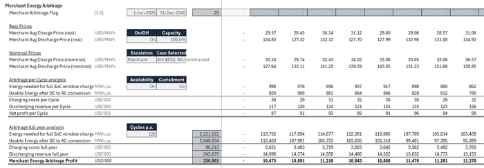

Step 1 — Start with a simple arbitrage switch (the flag)

The arbitrage flag is your on/off master switch. It keeps the model modular: you can run Case 5 with and without arbitrage and instantly see how much value is coming from merchant overlay versus contracted capacity. This is also what keeps the model audit-friendly—no hidden “merchant effects” lingering in formulas when the revenue stream is off.

Step 2 — Pull the price forecasts (charge and discharge) as time series

Arbitrage is driven by two annual price paths:

• Average charge price (what you pay to buy energy from the grid)

• Average discharge price (what you earn when selling back)

In a yearly model, you’re not trying to optimize hourly dispatch. You’re using forecast containers—typically provided by a market consultant—and consistently mapping them into cash flows. The important modeling discipline is traceability: your operations sheet should make it obvious which dropdown price case is selected and which rows in your time-dependent forecast table feed the revenue engine.

Step 3 — Convert real prices to nominal (indexation)

If your price forecast is “real” (today’s dollars), you still need to express cash flows in the model’s nominal currency framework. This is where index selection matters: the model multiplies real prices by the chosen escalation index, so your revenue and cost series stay consistent with inflation assumptions used across the rest of the project finance model.

Step 4 — Compute energy per cycle (charge energy vs discharge energy)

This is the core of “lender-clean” arbitrage modeling:

• Energy needed to charge (AC from grid)
  This is how many MWh you must buy to fully charge the usable state-of-charge window, after applying any availability/curtailment switches if you choose to reflect them explicitly.

• Energy delivered on discharge (AC to grid)
  This is how many MWh you can sell back after the efficiency chain and conversion losses—typically lower than charge energy because round-trip losses are real economics.

If you keep your boundary discipline straight (what lives on AC vs DC), your outputs will “feel right” instantly: charge energy is slightly higher than discharge energy, and the difference is your efficiency loss expressed in MWh.

Step 5 — Profit per cycle → profit per year

Once prices and energy are correct, the economics become simple:

• Charge cost per cycle = charge price × charge energy

• Discharge revenue per cycle = discharge price × discharge energy

• Net profit per cycle = revenue − cost
  Then scale it:

• Annual charge cost = charge cost/cycle × cycles/year

• Annual discharge revenue = revenue/cycle × cycles/year

• Annual arbitrage profit = annual revenue − annual cost

This is where your “spread story” becomes a decision-grade number. You can see exactly what drives merchant upside: spreads, losses, and throughput—nothing else.

Step 6 — Keep the RA constraint visible

Because this is Case 5 in our BESS Deal Lab (RA + Arbitrage), your cycles assumption is intentionally not “as many as possible.” The logic is: RA product first, arbitrage second. That’s the difference between a merchant model that looks great and a merchant model that looks credible.

Common Pitfalls and the Lender Lens (Keep It Underwriteable)

The fastest way to overstate BESS Merchant Energy Arbitrage is to treat a constrained battery like a free merchant trader. In practice, the “spread” is only one ingredient—and most modeling errors happen when assumptions quietly contradict the physical or commercial boundaries of the asset.

Here are the pitfalls that matter most:

• Too many cycles, not enough constraint. If the battery is committed to RA, you don’t get unlimited dispatch flexibility. Your cycles per year should reflect what’s actually left for arbitrage after contractual priorities are met. A conservative EFC assumption is often more credible than a “perfect daily cycle” assumption.

• Perfect price capture. Real-world arbitrage is not “charge at the daily minimum, discharge at the peak.” If your case is RA-constrained, your charge/discharge prices must reflect that constraint. Otherwise, your BESS Merchant Energy Arbitrage becomes an unrealistic upside story that won’t survive diligence.

• Ignoring losses (or applying them inconsistently). Your charge energy should be larger than your discharge energy once efficiencies and conversion losses are applied. If your model shows the opposite—or if it’s unclear where losses are captured—your BESS Merchant Energy Arbitrage math will be hard to defend.

• Debt vs equity credit is not the same. Even when merchant assumptions are reasonable, lenders often apply haircuts (for example, partial credit to merchant cash flows in debt sizing). That’s not “pessimism”—it’s credit discipline. Build your model so it’s easy to separate the equity view (full merchant upside) from the debt view (haircut merchant cash flows), and you’ll get a much cleaner investment committee narrative.

If you keep these guardrails in place, your merchant overlay will read like a financeable structure—not a trading strategy.

Wrap-Up and Next Steps (Deal Lab + RVA Certification)

You now have the full blueprint for modeling BESS Merchant Energy Arbitrage in a project finance-style Excel framework: price forecasts → cycles → energy per cycle (charge vs discharge) → profit per cycle → annual cash flows. When you layer that on top of a contracted RA base, the result is a structure that can be compared side-by-side across scenarios—without hand-waving.

If you want to follow along hands-on, the BESS Deal Lab (Project Pulse) walks through the full build inside Excel step-by-step, including the supporting reference materials and the dashboard outputs that make results decision-ready. And if you want broader mastery beyond this single revenue stack—covering storage, renewables, debt sizing logic, sensitivities, and investment-grade outputs—this content also ties into the wider RVA Certification Program, where you build repeatable project finance modeling skills across multiple real-world deal structures.