
Table of Contents
- Project Pulse in 90 Seconds (and what you’ll learn)
- Why AC vs DC Boundaries Decide Bankability
- Nameplate vs Usable Energy: Where Duration Breaks
- 1) Nameplate is the product you sold (AC at the POI)
- 2) Overbuild ratio: why DC is intentionally larger than AC
- 3) Usable energy is what physics allows (DC translated back to AC)
- 4) Effective duration is the KPI that reveals the break
- 5) What “breach” really means (in practical terms)
- 6) Why augmentation is the bridge (and why timing matters)
- How AC Deliverability Is Calculated (and Why It Drives Augmentation)
- How Augmentation Triggers Work (Headroom Threshold)
- 1) Headroom vs nameplate: the watchdog metric
- 2) Trigger threshold: why you must act before breach
- 3) Restore buffer: rebuilding headroom above the product
- 4) Sizing: translating an AC headroom target into DC cells installed
- 5) Timing mechanics: trigger year vs installation year
- 6) Augmentations degrade too (and revenue structure changes frequency)
- Deal Lab Part 3: Build the trigger + restore + sizing logic in Excel
- Closing Summary
- FAQs
A battery is sold as an AC product at the point of interconnection (POI): a defined power rating (MW) sustained for a defined duration (hours). The challenge is that the asset behind that product evolves over time. Degradation gradually reduces usable energy, which can quietly shrink deliverable duration until the project is no longer providing the product it originally contracted or underwrote. This is where BESS augmentation modeling becomes essential. Done properly, it forces boundary discipline: physics lives on the DC side, while cashflows and contractual deliverability settle on the AC side. The model’s job is to translate DC degradation into AC deliverability, and then schedule augmentation before you breach nameplate requirements.
In this article, you’ll learn how to think about AC vs DC deliverability the way investors and lenders do: nameplate obligations on the AC side, usable energy on the DC side, and augmentation as the bridge that keeps the asset “bankable” over its full life.
Project Pulse in 90 Seconds (and what you’ll learn)
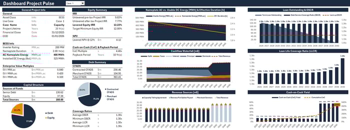
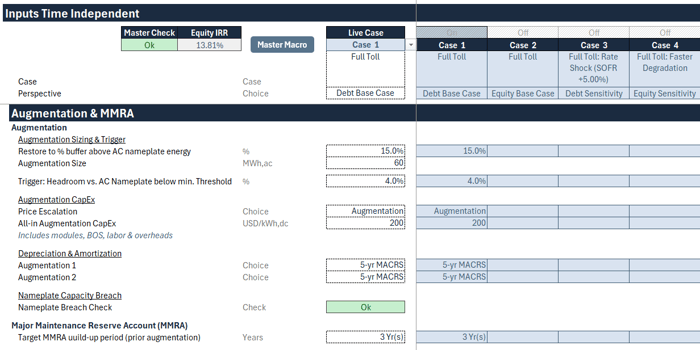
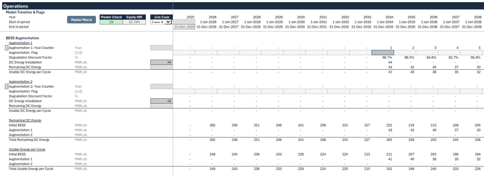
To make the concepts concrete, this article follows the lens of Project Pulse — a 200 MW,ac multi-duration BESS case study designed around one central question: how do different technical configurations and revenue structures change bankability, augmentation needs, and ultimately equity returns?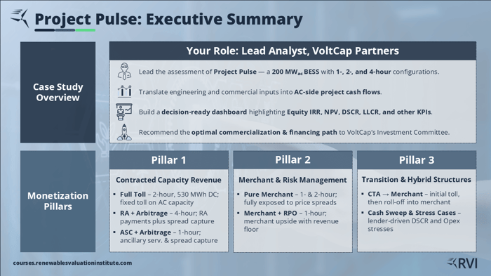 In the Deal Lab, you step into the role of a lead analyst assessing the project and turning engineering and commercial inputs into clean AC-side cashflows, a decision-ready dashboard, and a clear recommendation for an investment committee. The analysis is organized into three monetization pillars:
Pillar 1: Contracted capacity revenue — structures anchored in long-term capacity payments with varying levels of merchant upside.
Pillar 2: Merchant exposure and risk management — fully merchant cases and a revenue floor structure (a “put” style mechanism) designed to preserve upside while improving lender comfort.
Pillar 3: Transition and lender-driven structures — roll-off structures and more conservative credit-aligned mechanics (including stress and cash sweep style thinking).
Across these pillars, the objective is not just to “get an IRR,” but to understand why a given structure performs the way it does — and whether it remains deliverable at the POI over 20 years without breaking the product you sold.
Deal Lab Part 1 introduces Project Pulse, the three-pillar framework, and the overall modeling and dashboarding workflow that this article builds on.
Why AC vs DC Boundaries Decide Bankability
If there’s one principle that makes BESS Augmentation Modeling “lender-clean” and investor-grade, it’s boundary discipline: cash settles on the AC side, physics lives on the DC side. Most modeling mistakes happen when these boundaries get blurred—especially when analysts try to force technical battery behavior directly into AC cashflow logic without a transparent translation layer.
AC is the commercial boundary (what gets paid)
The AC side at the point of interconnection (POI) is where the outside world measures the asset:
Contracts define deliverables in MW,ac and hours (a 1-hour, 2-hour, or 4-hour product).
Market revenues settle on what you can inject at the POI.
Lenders finance what the project can reliably deliver to support debt-sizing metrics.
In other words, the POI is your cash register ceiling. If you can’t deliver at the POI, you can’t earn the revenue you modeled—no matter what the battery “still has” on the DC side.
DC is the technical boundary (what the battery actually does)
The DC side is where the battery’s physical reality sits:
installed energy and usable state-of-charge limits,
efficiency losses through the charge/discharge path,
degradation curves that reduce usable energy over time,
and augmentation campaigns that restore performance.
Degradation is not just a “technical input” to be filed away—it is a time-dependent reduction in the DC energy you can store and cycle, which must be translated back into AC deliverability to understand whether the product still holds.
This is why BESS Augmentation Modeling is best thought of as a bridge: you model degradation where it belongs (DC), and you test obligations where they exist (AC).
The translation layer: DC → AC deliverability
A disciplined model uses a transparent sequence:
Start with usable DC energy per cycle
After applying degradation and the usable state-of-charge window, you know how much DC energy is actually available in the cells.Convert to AC deliverable energy at the POI
Apply the discharge-side losses and efficiencies to translate DC energy into the MWh,ac that can be delivered back to the grid connection.Cap deliverability at nameplate obligations
Even if the battery could theoretically deliver more, the contract product is defined by POI power × duration. Deliverability is ultimately constrained by what the POI rating and duration represent in commercial terms.Express the result as effective duration
Effective duration is the clean KPI that ties everything together:
deliverable MWh,ac per cycle ÷ POI MW,ac.
If effective duration drifts below the contracted product, your model should not quietly accept the breach. It should surface it clearly—and that’s the moment BESS Augmentation Modeling enters the story.
A simple rule set (useful to keep models “lender-clean”)
Here’s the practical discipline that keeps the model readable and defensible:
Revenues and contractual tests belong on the AC side at the POI.
That’s the language of offtakers, markets, and credit committees.Degradation and augmentation belong on the DC side.
That’s the language of physics and equipment performance.Convert AC ↔ DC only to test deliverability and size augmentation.
The conversion is not cosmetic—it is the bridge between technical reality and commercial obligations.
This discipline is what prevents the most common failure mode: “stacking” revenues and assumptions in ways that double-count energy or hide the real deliverability constraint. When you respect the boundary, you get a model where augmentation is not an afterthought, but a transparent, testable mechanism that keeps the project’s AC product intact over time.
Nameplate vs Usable Energy: Where Duration Breaks
At the heart of BESS Augmentation Modeling is a simple but powerful comparison: what the market expects the battery to deliver versus what the battery can actually deliver as it ages.
1) Nameplate is the product you sold (AC at the POI)
Nameplate deliverability is the commercial definition of the asset:
POI power (MW,ac) is fixed by the inverter and interconnection.
Duration (hours) defines how long that POI power can be sustained.
Together, these define nameplate AC energy per cycle (MWh,ac).
This “nameplate” line is not a modeling preference — it is the benchmark embedded in contracts, performance expectations, and (implicitly or explicitly) in credit and valuation work. A 200 MW / 2-hour battery is not “about” DC cells; it is a promise to the market that the project can repeatedly deliver the required AC energy at the POI.
2) Overbuild ratio: why DC is intentionally larger than AC
Before we even talk about degradation, there’s a foundational design decision that explains why “usable” and “nameplate” are not the same thing: the overbuild ratio.
Most utility-scale BESS are intentionally built with more DC energy capacity than the AC side can export at the POI. In practical terms:
The POI defines how much power can flow to the grid (MW,ac).
The DC energy installed in the cells defines how much energy is available behind the inverter (MWh,dc).
The overbuild ratio is the design buffer that creates headroom between the two.
This matters because overbuild isn’t just “extra battery.” It is engineered headroom that helps the project:
absorb degradation while still delivering the contracted AC product,
respect usable state-of-charge limits (you typically don’t cycle 100% to 0%),
maintain deliverability once you layer in losses and efficiencies through the charge/discharge path.
In other words, overbuild is the first line of defense against duration shrinkage. But it is not infinite — it gets consumed as the battery degrades.
3) Usable energy is what physics allows (DC translated back to AC)
Now step behind the product. Over time, usable energy declines due to:
degradation (cycling and calendar aging reduce usable DC capacity),
SoC window constraints (you don’t operate from 100% to 0%),
losses/efficiencies in both charge and discharge paths.
In a disciplined model, those effects live on the DC side — then you translate them back into the deliverable MWh,ac at the point of interconnection. This is where BESS Augmentation Modeling becomes non-negotiable: if you only track DC capacity and never translate it into AC deliverability, you can miss the moment the asset stops behaving like the contracted product.
4) Effective duration is the KPI that reveals the break
Once you have deliverable MWh,ac per cycle, the key KPI is straightforward:
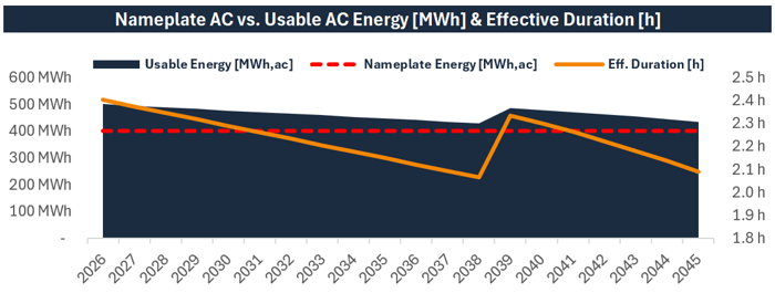
Effective Duration (hours) = Deliverable MWh,ac per cycle ÷ POI MW,acThis is why your dashboard view is so useful:
The dashed nameplate line is what the market expects.
The usable (deliverable) curve/area is what the asset can actually provide after degradation, SoC limits, and losses.
The effective duration line translates that gap into a single, intuitive number.
In early years, overbuild often creates visible headroom: usable deliverability can exceed the nameplate requirement. But as degradation accumulates, that headroom erodes. Eventually, the effective duration approaches the point where the system is at risk of falling below the product definition. That’s the inflection point where BESS Augmentation Modeling stops being a technical detail and becomes a commercial constraint.
5) What “breach” really means (in practical terms)
When usable deliverability falls below nameplate requirements, you have a mismatch between:
what the project is obligated to provide (the product you sold), and
what the aging system can reliably deliver.
Even without going deep into contract language, the consequence is intuitive: the project is no longer delivering the contracted duration, which can translate into performance shortfalls, reduced revenues, or penalties depending on the structure. More importantly, it undermines the stability assumptions that debt sizing and valuation are built on.
6) Why augmentation is the bridge (and why timing matters)
Overbuild buys you time — but it doesn’t eliminate the problem. Once degradation consumes enough headroom, the model needs a bridge back to bankable deliverability. That bridge is augmentation.
The “jump” you see in deliverable energy and effective duration is not cosmetic — it is the model reflecting new cells installed to rebuild headroom above nameplate.
And this is the key insight investors often underestimate:
Augmentation frequency is not fixed. It is commercially driven.
A merchant-heavy dispatch profile can accelerate degradation and pull augmentation forward (or require more campaigns), while a more stable contracted structure may preserve headroom for longer.
In the next section, we’ll formalize this moment into a repeatable, lender-clean decision rule: a headroom threshold that triggers augmentation before breach, ensuring the project continues to deliver the AC product it sold at the POI.
How AC Deliverability Is Calculated (and Why It Drives Augmentation)
Everything in BESS Augmentation Modeling becomes much clearer once you treat deliverability as a measured AC outcome rather than a vague “battery health” concept. The goal is not to track degradation in isolation—it’s to answer one investment-grade question year by year:
How many MWh can the BESS actually deliver at the POI each cycle, and what effective duration does that translate into?
That deliverability calculation is the bridge between DC physics and AC bankability.
1) Start from usable DC energy (the physics side)
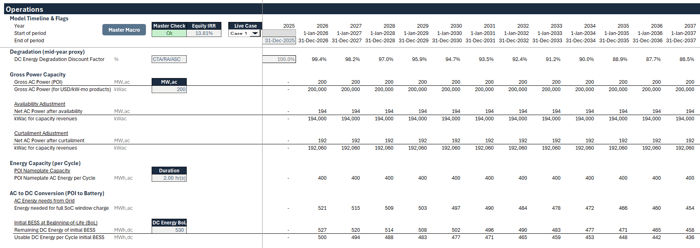
By this point in the logic, you already have the battery’s usable DC energy per cycle after:
degradation has reduced the remaining DC capacity,
the usable state-of-charge window has capped what can actually be cycled,
and the model reflects the “behind-the-meter” reality of the cells.
This is where many models stop—and that’s precisely where bankability risk gets hidden. BESS Augmentation Modeling requires the next step: translating that DC energy into what the grid can actually receive.
2) Convert DC → AC through the discharge path
To move from usable DC energy to deliverable AC energy at the POI, you pass through the discharge-side efficiency chain:
discharge conversion efficiency in the power conversion system (PCS),
transformer and medium-voltage losses between inverter and POI.
This step is conceptually simple but critical: it ensures your model’s deliverability is expressed in the same unit the market pays on—MWh,ac at the POI. In other words, it keeps BESS Augmentation Modeling aligned with how contracts and dashboards should be read.
3) Cap deliverability at the nameplate product
Now you have two relevant quantities:
Nameplate AC energy per cycle (what the product definition implies): POI MW,ac × contracted duration
Physically deliverable AC energy (what the battery can truly output after degradation and losses)
A bankable model does not assume the project can deliver “whatever the battery has.” It caps deliverability at the product boundary using a simple logic: deliverable energy is the minimum of nameplate obligation and physical capability.
This is also where the story becomes actionable: the first year may show surplus headroom, but later years can show a shortfall that creeps in quietly until the asset is about to violate the product definition. This cap-and-compare logic is one of the cleanest ways to keep BESS Augmentation Modeling transparent and audit-friendly.
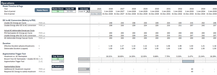
4) Translate deliverable energy into effective duration
Once deliverable MWh,ac per cycle is known, effective duration is simply:
Effective Duration (hours) = Deliverable MWh,ac ÷ POI MW,ac
This is the KPI you can put in front of an investment committee without caveats. It collapses all the DC complexity into one AC deliverability metric: “how many hours does this battery still behave like the product we sold?”
And this is exactly why effective duration naturally becomes the input into augmentation logic: when duration approaches the contractual floor, you must either restore headroom or accept commercial and financing consequences. In BESS Augmentation Modeling, the augmentation trigger is not arbitrary—it is the direct response to an approaching deliverability failure.
Deal Lab Part 2: Nameplate vs usable energy → effective duration in Excel
This walkthrough shows the full logic chain: usable DC energy → AC deliverability at the POI → nameplate cap → effective duration.
How Augmentation Triggers Work (Headroom Threshold)
Once you’ve translated DC physics into AC deliverability, BESS Augmentation Modeling becomes a decision-rule problem: when should the project install new cells, and how early should that decision be made to avoid commercial breach?
The cleanest way to do this—especially in lender-style models—is to monitor headroom versus AC nameplate. Headroom is the buffer between what the project can physically deliver at the POI and what the contracted “product” requires.
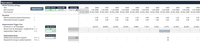
1) Headroom vs nameplate: the watchdog metric
Headroom is computed directly from AC deliverability:
Deliverable AC energy per cycle (after DC→AC conversion)
divided byNameplate AC energy per cycle (POI MW,ac × contracted duration)
Then subtract 1 to express the result as “buffer” rather than a ratio.
If the battery can deliver 120% of nameplate, headroom is +20%. As degradation accumulates, headroom declines. When it approaches zero, the asset is about to stop behaving like the product it sold.
This metric is powerful because it is:
AC-based (so it aligns with contracts, dashboards, and bankability),
directly interpretable (a single percentage buffer), and
structurally tied to the augmentation decision.
That’s why in BESS Augmentation Modeling, headroom is the natural trigger signal—more defensible than arbitrary calendar-based replacement assumptions.
2) Trigger threshold: why you must act before breach
A key modeling insight is that augmentation should not be triggered when the project is already in breach. By the time headroom is negative, you’re already failing the product definition.
Instead, you define a minimum headroom threshold (for example, a few percentage points). Once headroom drops below that threshold, the model flags a trigger.
Conceptually, this threshold is a risk posture:
A higher threshold triggers earlier (more conservative, more “credit-aligned”).
A lower threshold triggers later (more aggressive, may increase breach risk under volatility or imperfect execution).
So BESS Augmentation Modeling is not just “do we augment?”—it’s “how conservative is our deliverability policy?”
3) Restore buffer: rebuilding headroom above the product
When augmentation occurs, you typically don’t restore to exactly nameplate deliverability. You restore above it—because if you climb back to the minimum, you will trigger again too quickly.
This is where the second key input comes in: restore-to buffer above nameplate (often expressed as a percentage). It defines how much headroom you want immediately after an augmentation event.
This is the bridge between initial design headroom (your overbuild ratio early in life) and “recreated” headroom later in life. In BESS Augmentation Modeling, augmentation is effectively a mechanism to replenish the buffer that degradation steadily consumes.
4) Sizing: translating an AC headroom target into DC cells installed
The restore buffer is defined in AC terms (because that’s the product boundary). But the installation is a DC energy decision (because you install cells).
So the model needs a clean translation:
Determine the additional MWh,ac needed to restore the target headroom above nameplate.
Convert that AC requirement into a DC MWh installation amount using the project’s AC↔DC conversion relationship (loss-adjusted).
This keeps the sizing logic transparent: you’re not “guessing a DC add”—you’re installing exactly what is required to restore AC deliverability after accounting for losses.
5) Timing mechanics: trigger year vs installation year
A lender-clean implementation usually separates:
the year in which the deliverability risk becomes visible (trigger),
and the year in which augmentation is installed (event).
This avoids circularity and reflects real execution: you detect shrinking headroom, commit to augmentation, and then install it in the following period. In BESS Augmentation Modeling, that separation is what turns an intuitive concept into a robust time series.
6) Augmentations degrade too (and revenue structure changes frequency)
Once installed, augmentation energy begins degrading as well. That means the model needs:
an augmentation “year counter” (so degradation curves apply from year 1 of the new cells),
and the ability for a second augmentation to occur if the revenue structure is highly cycling-intensive.
This is where your commercial story becomes concrete: a merchant-heavy strategy can accelerate degradation and pull augmentations forward or increase the number of campaigns, while a stable contracted tolling structure may require fewer.
Deal Lab Part 3: Build the trigger + restore + sizing logic in Excel
This walkthrough implements the full augmentation mechanics from scratch: headroom calculation → threshold trigger → restore buffer sizing → installation event → validation that nameplate breach is avoided.
Closing Summary
At its core, BESS Augmentation Modeling is about keeping the product you sold to the market intact over time. The discipline is simple: physics lives on the DC side, cash and contractual deliverability settle on the AC side at the POI, and augmentation is the bridge that restores headroom before a nameplate breach turns into a commercial and financing problem. When you model that translation cleanly—usable DC energy → AC deliverability → effective duration → trigger and restore logic—you end up with outputs that are not only technically correct, but also investor- and lender-grade.
If you’d like to follow this hands-on in Excel, the BESS Deal Lab (Project Pulse) walks through the full model build step by step, including the Project Pulse Information Memorandum, the start file, and the BESS Secret Sauce reference guide—so you can mirror the exact workflow and logic covered in this article.

And if you want the broader, structured path to mastering renewable energy project finance modeling beyond a single case study, the RVA Certification Program gives you access to the full curriculum across projects, structures, and difficulty levels—so you can build durable, repeatable modeling skills and apply them across real transactions.
FAQs
What is BESS Augmentation Modeling, and why does it matter in project finance?
BESS Augmentation Modeling is the process of translating battery degradation on the DC side into AC deliverability at the point of interconnection (POI)—and then scheduling and sizing augmentation (new battery cells) so the project continues to deliver the contracted product (e.g., a 1-hour or 2-hour battery) over its full life.
It matters in project finance because lenders and offtakers ultimately care about what can be delivered and monetized on an AC basis at the POI. As the battery degrades, the usable energy per cycle declines, which reduces effective duration and can eventually cause the project to fall below its nameplate deliverability. If a model ignores this mechanism (or treats augmentation as a generic, flat assumption), it can materially misstate:
whether the project remains bankable under contracted obligations,
how many augmentation campaigns are needed (and when), and
the resulting impact on cashflows, DSCR/LLCR, and equity returns.
In short: augmentation is the bridge between what the market expects the battery to deliver and what the battery can physically deliver over time—and modeling it cleanly is essential for investor- and lender-grade analysis.
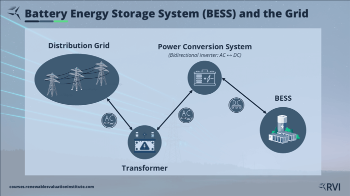
What’s the difference between AC and DC in a BESS financial model—and why do revenues “settle” on the AC side?
In a utility-scale BESS, DC is the battery’s internal world (the cells and stored energy), while AC is the grid-facing world (what flows through the inverter and across the point of interconnection).
DC side (physics): installed energy capacity (MWh,dc), degradation, usable state-of-charge limits, and the energy that actually exists inside the battery.
AC side (commercial reality): deliverable power and energy at the POI, which defines what contracts require and what markets pay for (MW,ac and MWh,ac).
Revenues “settle” on the AC side because the grid and counterparties can only measure and pay based on what is injected or withdrawn at the POI. That’s the boundary that defines:
contracted products (e.g., “200 MW for 2 hours”),
dispatch deliverability, and
what lenders finance in terms of sustainable cash generation.
A lender-clean model, therefore, keeps strict boundary discipline: it models degradation where it belongs (DC), then translates DC energy into AC deliverability using the efficiency/loss chain. That AC deliverability is what should drive effective duration, nameplate comparisons, and ultimately augmentation timing and sizing.
What is “effective duration,” and how is it different from nameplate duration?
Nameplate duration is the product definition: it’s what the battery is marketed, contracted, or underwritten as delivering at the POI—typically POI MW,ac × hours (e.g., 200 MW for 2 hours = 400 MWh,ac per cycle).
Effective duration, by contrast, is what the asset can actually deliver at the POI after you account for real-world constraints over time, including:
degradation reducing usable capacity,
usable state-of-charge limits,
charge/discharge efficiency and transformer/MV losses.
In a clean model, effective duration is calculated from deliverability on the AC side:
Effective Duration (hours) = Deliverable MWh,ac per cycle ÷ POI MW,ac
Early in life, effective duration is often above nameplate because systems are designed with buffer (including DC overbuild and conservative operating limits). But as degradation accumulates, effective duration declines. When it approaches—or falls below—nameplate duration, the battery is at risk of no longer delivering the contracted product. That’s why effective duration is one of the most practical “watchdog” KPIs in bankability-focused BESS modeling and the natural input into augmentation trigger logic.
What is the overbuild ratio, and how does it affect deliverability and augmentation needs?
The overbuild ratio describes how much DC energy capacity is installed relative to what the AC side can deliver at the point of interconnection. In simple terms, it reflects that most BESS are intentionally built with more DC energy “behind the inverter” than the AC product would suggest.
That design choice matters because overbuild creates initial headroom that helps the project:
respect usable state-of-charge limits (you typically don’t cycle 100% to 0%),
absorb efficiency losses through the charge/discharge path, and
tolerate degradation while still meeting the AC nameplate product (MW at the POI for a given duration).
However, overbuild is not a permanent solution—it’s a buffer that gets consumed over time as degradation reduces usable DC capacity. Once enough headroom is eroded, effective duration approaches the contractual floor and the project must either:
accept reduced deliverability (often not feasible under contracted products), or
install new cells to restore headroom through augmentation.
So the practical takeaway is: the overbuild ratio can delay the first augmentation, but it does not eliminate augmentation. The more aggressively the battery is cycled (e.g., merchant-heavy operation), the faster that headroom gets used up and the more important augmentation timing and sizing become.
How do you decide when to trigger augmentation in a BESS model? Answer:
A robust approach is to trigger augmentation based on headroom versus AC nameplate deliverability, not on a fixed calendar schedule. The reason is simple: the need for augmentation depends on how quickly the battery’s usable capacity is consumed—which is driven by degradation, operating strategy, and the revenue stack.
A lender-clean trigger method typically works like this:
Calculate deliverable AC energy per cycle at the POI
Start with usable DC energy (after degradation and SoC window), then convert DC → AC using discharge-side efficiencies and losses.Compare deliverable AC energy to nameplate AC energy per cycle
Nameplate is POI MW,ac × contracted duration. Compute headroom as:
Headroom = (Deliverable MWh,ac ÷ Nameplate MWh,ac) − 1Define a minimum headroom threshold
If headroom drops below a set level (e.g., a few percentage points), the model flags an augmentation trigger. This ensures you act before you fall into breach.Separate trigger timing from installation timing
Many models trigger in one year and install in the next to avoid circularity and to reflect practical execution.
This approach is preferred because it is transparent and aligns with commercial reality: augmentation happens when the asset is about to stop delivering the contracted product—not simply because a certain number of years have passed.
How do you size augmentation in a BESS model (restore logic)?
Sizing augmentation is the step that turns a “we should augment” signal into a quantified DC energy installation plan that restores the project’s AC deliverability at the POI. A clean, investor-grade method typically follows four moves:
Set a restore-to buffer above nameplate
Instead of restoring to exactly nameplate deliverability (e.g., exactly 2.0 hours), you restore to a buffer above nameplate (often expressed as a %). This rebuilds headroom so you don’t trigger another augmentation immediately after the first one.Convert the restore target into an additional AC energy requirement
Start with the nameplate AC energy per cycle (POI MW,ac × contracted duration).
Then compute the additional MWh,ac you want as buffer (e.g., 15% of nameplate).Translate required MWh,ac into required MWh,dc installed
This is the core translation step. Because you install cells on the DC side, you need a conversion factor that reflects the project’s AC↔DC relationship (including relevant losses/efficiencies). Practically, you use the model’s existing energy conversion logic to answer:
“To deliver X additional MWh,ac at the POI, how many MWh,dc do I need behind the inverter?”
This keeps the sizing transparent and consistent with the deliverability calculations you already trust.
Apply augmentation degradation over time (and allow multiple campaigns if needed)
New cells degrade too, so the model should apply an augmentation-specific degradation curve that starts in year 1 of the augmentation, not year 1 of the project. That’s why many lender-clean models use an augmentation year counter. If the operating strategy is cycling-intensive (often the case in merchant-heavy scenarios), the first augmentation may not be enough, and the model may correctly trigger a second campaign later in the asset life.
The key takeaway: augmentation sizing is not a guess or a fixed % of initial capacity. It’s a deliverability-driven design choice—restore headroom above nameplate on an AC basis, then translate that requirement into DC cells installed in a way that is consistent with your efficiency and loss chain.
What is the BESS Deal Lab (Project Pulse), and what do I get if I enroll?
The BESS Deal Lab (Project Pulse) is a hands-on case study where you build and analyze a 200 MW multi-duration BESS project finance model the way an investment team would: starting from technical and commercial inputs, translating them into lender-clean AC-side cashflows, and ending with a decision-ready dashboard that supports an investment committee recommendation.
When you enroll, you’re not just getting a conceptual explanation—you’re following a structured workflow with the core materials needed to replicate the analysis in Excel, including:
the Project Pulse model files (so you can mirror the build step by step),
the Project Pulse Information Memorandum (the deal context and assumptions),
and the BESS Secret Sauce reference guide (the modeling “rules” and frameworks behind the mechanics).
The Deal Lab is designed to help you internalize the real-world logic behind topics like AC vs DC deliverability, effective duration, and augmentation trigger and restore sizing—and then apply the same discipline across different revenue stacks and structuring choices. If this blog post clicked for you and you want to implement the mechanics yourself rather than just read about them, the Deal Lab is the fastest way to do it.
How does the RVA Certification Program relate to the BESS Deal Lab—and who is it for?
The RVA Certification Program is the broader, structured learning path designed to build complete, job-relevant competency in renewable energy project finance modeling and valuation—not just for one technology or one case study. Think of the BESS Deal Lab (Project Pulse) as a deep, hands-on application module, while the RVA Certification Program is the full curriculum that ties together fundamentals, modeling mechanics, and advanced deal structuring across the wider renewable landscape.
It’s for professionals who want more than isolated lessons or one-off templates—especially if you want a repeatable skill set you can apply across transactions, interviews, and day-to-day work. Depending on where you are today, the RVA path typically helps you:
build strong foundations (how energy projects make money, core modeling structure, key metrics),
develop advanced modeling discipline (bankability logic, scenario analysis, financing structures), and
apply those skills to realistic case studies like the Deal Lab—so you can defend your outputs with investor-grade reasoning.
If your goal is to go beyond “I followed a model once” to “I can build, analyze, and explain these projects confidently,” the RVA Certification Program is the umbrella that gives you access to the full progression and lets you choose the courses and case studies that match your goals and experience level.