
Table of Contents
- Real-World Case Study: Modeling P-Values in Excel
- The Statistical Theory Behind P-Values in Renewable Energy
- Why Sponsors and Lenders Think Differently About P50 vs. P99
- Energy Yield Assessments (EYA) – Where P50 and Uncertainty Come From
- How to Model P50, P75, P90, and P99 Using Only P50 and Uncertainty
- From Theory to Practice: Applying P50 vs. P99 in Real Models
- FAQs
How to model P50, P75, P90, P99, or any other P-value is a fundamental skill for anyone building bankable renewable energy project finance models. These statistical confidence levels aren’t just academic metrics — they determine how much debt a project can raise, how equity returns are shaped, and how resilient cash flows will be under different production outcomes.
In practice, lenders and equity investors use different P-values to assess risk and opportunity. The ability to calculate and incorporate multiple P-values into a single model is a hallmark of advanced financial modeling — and it’s often a topic that comes up in real project finance deals as well as in competitive modeling tests.
Real-World Case Study: Modeling P-Values in Excel
To see this in action, let’s look at a recent case study that demonstrates how to model any P-value using just two key inputs: the P50 energy yield and the uncertainty (standard deviation) of production, both typically provided in an Energy Yield Assessment (EYA).
In the full video walkthrough below, you’ll see exactly how to implement this in Excel using the NORM.INV function — a quick, reliable way to generate P75, P90, P99, or any other P-value for your analysis. This example is taken from our advanced modeling curriculum, where we integrate these yield scenarios directly into debt sizing and IRR calculations.
📺 Watch the step-by-step breakdown:
How to Interpret P-Values in Energy Yield Analysis
In renewable energy project finance, P-values are a statistical way of expressing production uncertainty. They indicate the probability that actual energy generation will meet or exceed a certain level in a given year.

For example:
P50: There’s a 50% probability that annual production will be at this level or higher.
P90: There’s a 90% probability that annual production will be at this level or higher. In other words, in 9 out of 10 years, actual generation is expected to meet or exceed the P90 value.
P99: Extremely conservative, representing a 99% probability of achieving at least this amount of production.
When learning how to model P50 and other P-values in Excel, it’s important to understand that lower P-values (e.g., P50) reflect higher expected generation but also carry more risk of underperformance. Higher P-values (e.g., P90, P99) are more conservative, ensuring higher confidence but at the cost of lower expected output.
The Statistical Theory Behind P-Values in Renewable Energy
P-values in renewable energy modeling are rooted in probability theory and statistics. They quantify the likelihood that a certain level of annual energy production will be met or exceeded, based on historical weather and resource data.
For wind and solar projects, production depends heavily on natural variability — wind speeds for turbines and solar irradiance for PV systems — which fluctuate from year to year. Over long timeframes, these variations tend to follow a normal distribution (bell curve), shown below:
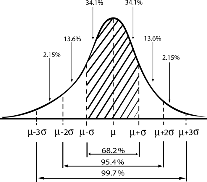
In this curve:
μ represents the mean (average) annual production.
Median (P50) is exactly at the center of the distribution — meaning there’s a 50% probability that the actual production will be higher, and 50% that it will be lower.
The standard deviation (σ) measures the spread of values around the mean.
Confidence Intervals and What They Mean
The percentages under the curve represent confidence intervals — the likelihood that actual production falls within a certain range of the mean:
±1σ: About 68.2% of the time, production will be within one standard deviation of the mean.
±2σ: About 95.4% of the time, production will be within two standard deviations.
±3σ: About 99.7% of the time, production will be within three standard deviations.
This is why the industry can confidently define other P-values such as P75, P90, and P99 — they correspond to specific points on this distribution. For example, P90 is the value that will be reached or exceeded 90% of the time (only 10% of years will have lower production).
When learning how to model P50, P75, P90, P99, or any other P-value, understanding this statistical foundation is essential. The normal distribution provides a consistent method to transform resource uncertainty into quantifiable production scenarios for both equity and debt analysis.
In practice, this framework allows modelers to apply just two key inputs — P50 and the standard deviation — to estimate any P-value with precision. It’s the bridge between resource variability and the financial models used by sponsors, lenders, and investors.
Why Sponsors and Lenders Think Differently About P50 vs. P99
Even when using the exact same P-values, equity investors (sponsors) and debt providers (lenders) often arrive at very different conclusions about how much debt a project should take on. This difference comes down to risk appetite and cash flow priorities.
The Sponsor’s Perspective – Optimizing Returns
Sponsors typically focus on maximizing equity IRR while keeping debt service obligations manageable. For them:
The P50 case is often the “base case” for evaluating returns.
If the project can comfortably service debt under P50 assumptions, sponsors may push for higher leverage to reduce upfront equity contributions.
They are willing to accept more variability in actual results, as long as the long-term average supports their return targets.
The Lender’s Perspective – Protecting Downside
Lenders are far more concerned about worst-case scenarios. Their primary objective is to ensure that debt service can be met even in low-production years.
They often size debt to a P99 or P90 production case with a lower DSCR target (e.g., 1.0x for P99, 1.2x for P90).
By testing multiple production scenarios side-by-side, lenders ensure that cash flow shortfalls in weaker years won’t trigger defaults.
Why This Matters in Modeling
If you’re learning how to model P50, P75, P90, and P99 cases in Excel, you must understand how each party interprets them:
Sponsors may see P50 as the driver for leverage and IRR optimization.
Lenders will use P99 (or P90) as a constraint to reduce leverage if downside scenarios can’t support target DSCRs.
In practice, this often results in dual debt-sizing constraints:
P50-based DSCR target
P99-based DSCR target
The more conservative outcome between these two will determine the final debt quantum — and it’s not always the P99 that results in a lower allowable debt quantum.
If you’re preparing for a modeling test or real-world project finance role, being able to explain why the two sides view P-values differently is just as important as calculating them. We cover exactly how to implement these dual constraints in our course How to Ace the Toughest Project Finance Modeling Tests.
Energy Yield Assessments (EYA) – Where P50 and Uncertainty Come From
Before modeling any P-value, it’s important to understand where the numbers actually come from. In project finance, these figures are typically provided in an Energy Yield Assessment (EYA) prepared by a Technical Advisor or Independent Engineer.
The EYA is a detailed report that estimates how much electricity a project will generate over its lifetime, based on:
Site-specific resource data (e.g., wind speeds from met masts, solar irradiance from pyranometers)
Turbine or PV module specifications and power curves
Loss factors such as shading, downtime, degradation, and electrical efficiency
Climate adjustments to account for long-term variability
The Role of P-values in the EYA
The EYA doesn’t just give one single number — it provides a distribution of expected annual production.
P50 is the mean of that distribution and represents the “most likely” long-term annual energy yield.
P90, P99, etc. are lower percentiles, showing how much production is exceeded in 90% or 99% of years.
The report will also specify the uncertainty in the energy yield, often expressed as a standard deviation. This is the second critical input (alongside P50) when learning how to model P50, P75, P90, or P99 in Excel.
Why Lenders Scrutinize the EYA
Lenders pay close attention to the methodology and assumptions in the EYA because:
A higher uncertainty means a wider spread between P50 and P99.
Conservative adjustments (like additional loss factors) can materially reduce available debt capacity.
The EYA is therefore not just a technical document — it’s a key driver in financial negotiations. If the uncertainty value is large, the P99 production case might be significantly lower than P50, and understanding how to model P50 alongside other P-values can reveal when it becomes a binding constraint in the debt-sizing process.
How to Model P50, P75, P90, and P99 Using Only P50 and Uncertainty
To reliably forecast a normal distribution of estimated energy yield, all you need is:
The median of the distribution — the P50 value (average annual generation).
The uncertainty — the standard deviation of the distribution, usually given in % terms in the Energy Yield Assessment (EYA).
With these two inputs, you can model any other P-value — P75, P90, or even P99 — using Excel’s NORM.INV function. This approach works because production variability in wind and solar projects closely follows a normal distribution over the long term.
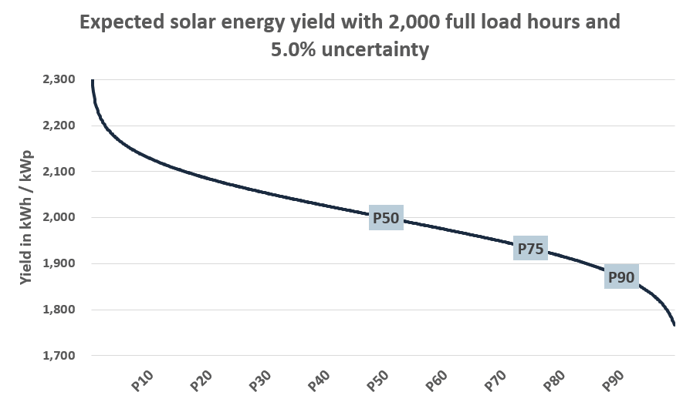
Practical Example from the Table
In the example below, the P50 is 2,000 MWh/MWp, and the uncertainty is 5% (100 MWh/MWp).
| Metric | Units | Value |
|---|---|---|
| P50 | MWh/MWp | 2,000 |
| Uncertainty | % | 5% |
Exemplary P90 Calculation:
=NORM.INV(1 - 0.90, 2000, 100)
Result: 1,872 MWh/MWp — meaning the plant will produce this amount or more in 90% of years.

Why This Matters
Knowing how to model P50, P75, P90, or P99 quickly and accurately is essential for stress-testing financial models under different resource conditions. It allows analysts to adjust debt sizing, evaluate equity returns, and simulate worst-case scenarios without re-building entire models from scratch.
From Theory to Practice: Applying P50 vs. P99 in Real Models
Understanding how to model P50, P75, P90, or P99 is only part of the challenge. In real-world project finance, you’ll need to integrate these scenarios into a full financial model — adjusting CFADS, running dual DSCR constraints, sculpting debt, and interpreting how each case impacts equity IRR and lender comfort.
Lenders will often require you to size debt using the more conservative outcome between the P50 and P99 cases, meaning you need to calculate both resulting debt quantums and understand which one constrains leverage. Equity investors, on the other hand, will be more focused on how these production scenarios influence long-term returns.
Master This Skill in Excel
If you’re preparing for a project finance modeling test, or simply want to apply this in your day-to-day role, the best way to cement your understanding is through hands-on practice:
How to Ace the Toughest Project Finance Modeling Tests – Advanced training on building, stress-testing, and explaining models in interviews.

RVA Certification Program – Full access to all courses, including deep dives on debt sculpting, energy yield scenarios, and lender/equity perspectives.
Both programs use real case studies where you’ll build P50 and P99 cases side-by-side, implement dual DSCR constraints, and optimize for both lender and sponsor requirements.
Final Takeaway
Knowing the statistical theory is important — but being able to model it cleanly in Excel and explain it confidently is what makes a real difference. Mastering how to model P50, P75, P90, or P99 will not only prepare you for interviews but also equip you to handle the kind of real-life modeling challenges that separate junior analysts from top-tier project finance professionals.
FAQs
What does P50, P75, P90, and P99 mean in energy yield modeling?
In renewable energy project finance, these P-values represent different confidence levels in production forecasts. For example, P50 means there is a 50% probability that annual energy production will meet or exceed the forecasted value — it’s effectively the “expected” or median scenario. P90 means production will be at that level or higher in 90% of cases (9 out of 10 years), making it a more conservative estimate. P99 is even more conservative, used by lenders to stress-test downside performance in debt sizing. Understanding these terms is key when learning how to model P50, P75, P90, and P99 energy yields in Excel.
How can I calculate any P-value, like P99, from a P50 and uncertainty value?
Any P-value (P75, P90, P99, etc.) can be derived in Excel if the P50 energy yield and the standard deviation (uncertainty) of production are known. These inputs are typically provided in the project’s Energy Yield Assessment (EYA) by the technical advisor or independent engineer.
Using Excel’s NORM.INV function, you can plug in:
Probability (e.g., 0.99 for P99, 0.9 for P90, 0.75 for P75)
Mean (the P50 value)
Standard Deviation (the uncertainty)
Excel then returns the energy yield for that P-value. This works because renewable energy resources like wind and solar follow a near-normal distribution over long-term averages.
We cover the exact step-by-step process in both Excel DNA for Project Finance Modeling (ideal if you’re building a solid modeling foundation) and How to Ace the Toughest Project Finance Modeling Tests (for advanced debt-sizing and multi-scenario builds).
Why do lenders often prefer P99 while equity investors focus on P50?
Lenders prioritize downside protection. A P99 energy yield means that in 99% of modeled years, production will be at or above that level — making it a conservative assumption for debt sizing. This helps ensure the project can still meet debt service obligations even in low-production years.
Equity investors, on the other hand, usually focus on P50 because it reflects the expected long-term average energy yield. Since their returns come after debt is serviced, they want to see the potential upside as well as realistic cash flow forecasts.
The difference in focus creates natural tension in negotiations — lenders push for resilience, while equity seeks to maximize leverage and IRR.
If you want to learn how to model both cases side by side and see how they impact debt capacity, our courses Excel DNA for Project Finance Modeling and How to Ace the Toughest Project Finance Modeling Tests cover real-world examples and hands-on Excel builds.
How should I prepare for a modeling test that involves P50 vs. P99 debt sizing?
Start by making sure you can confidently calculate CFADS (Cash Flow Available for Debt Service) under multiple production scenarios. Then, learn how to apply dual DSCR constraints so you can size debt based on both P50 and P99 cases, selecting whichever is more conservative.
A good approach is to:
Build a base model with clean, modular inputs.
Set up scenario toggles for different P-values.
Use Excel functions like NORM.INV to calculate any P-value given the P50 and standard deviation from the Energy Yield Assessment.
Sculpt debt service to meet target DSCRs in both cases.
For a structured path:
Begin with Excel DNA for Project Finance Modeling to master model setup and best practices.
Then move on to How to Ace the Toughest Project Finance Modeling Tests for advanced scenario modeling and interview-level case studies.
This progression will give you both the technical skills and the ability to explain your logic — which is key in passing high-level modeling assessments.
Why is the NORM.INV function useful for modeling P50, P75, P90, and P99 values in Excel?
The NORM.INV function in Excel allows analysts to calculate any P-value in a normally distributed dataset — which is why it’s widely used in energy yield modeling for solar and wind projects.
By inputting just two values from the Energy Yield Assessment — the P50 production estimate (mean) and the standard deviation (uncertainty) — NORM.INV can generate P75, P90, P99, or any other percentile.
For example:
=NORM.INV(0.90, P50_MWh, StdDev_MWh)
This formula returns the P90 production value, meaning the project is expected to produce at least this amount of energy in 90% of years.
This approach ensures consistent, transparent, and reproducible calculations when sizing debt or stress-testing financial models under multiple production scenarios.
If you want to practice applying NORM.INV in real project finance case studies, both Excel DNA for Project Finance Modeling and How to Ace the Toughest Project Finance Modeling Tests provide step-by-step examples.
What are the benefits of enrolling in the RVA Certification Program?
The Renewables Valuation Analyst (RVA) Certification Program is a one-stop shop for becoming a highly skilled, industry-ready project finance analyst in the renewable energy sector.
By enrolling, you gain:
Comprehensive coverage of both equity and debt perspectives — from core financial modeling skills to advanced scenario analysis.
Hands-on practice through multiple real-world case studies.
Lifetime access to all current and future courses in the program, so your skills stay sharp as the industry evolves.
Practical tools & templates used by professionals in leading banks, IPPs, and advisory firms.
Step-by-step learning path that takes you from foundational modeling (Excel DNA for Project Finance Modeling) to advanced structuring (Expert-Level Project Finance Modeling for Renewable Energy).
The RVA Certification Program is designed for anyone who wants to excel in interviews, hit the ground running in their role, and stand out as a go-to modeling expert in renewable energy project finance.